序列模型学习笔记

摘要：RNN, GRU, LSTM

1 RNN

1.1 前向传播

对于序列数据，使用标准神经网络存在以下问题：

• 对于不同的示例，输入和输出可能有不同的长度，因此输入层和输出层的神经元数量无法固定。
• 从输入文本的不同位置学到的同一特征无法共享。
• 模型中的参数太多，计算量太大。

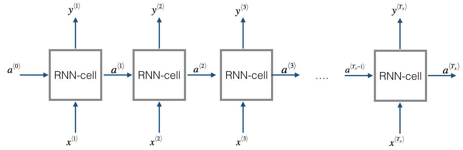
为了解决这些问题，引入循环神经网络（Recurrent Neural Network，RNN）。一种循环神经网络的结构如下图所示：

RNN的网络结构和神经网络一样，里面有很多神经元，较神经网络而言，每层都有两个输入，一个为上一层的输出，一个为新的输入。并且有2个输出。

一个时间序列就是一层神经网络。一个rnn处理1000个时间序列的数据集，这就是一个1000层的神经网络。

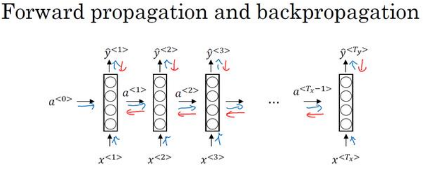
零时刻需要构造一个激活值a(0)，最常用的是零向量，也可以随机初始化。

.png)

当元素 x⟨t⟩输入对应时间步（Time Step）的隐藏层的同时，该隐藏层也会接收来自上一时间步的隐藏层的激活值 a⟨t−1⟩，其中 a⟨0⟩ 一般直接初始化为零向量。一个时间步输出一个对应的预测结果 y^⟨t⟩。

循环神经网络从左向右扫描数据，同时每个时间步的参数也是共享的，输入、激活、输出的参数对应为 Wax 、Waa、Wya。

下图是一个 RNN 神经元的结构：

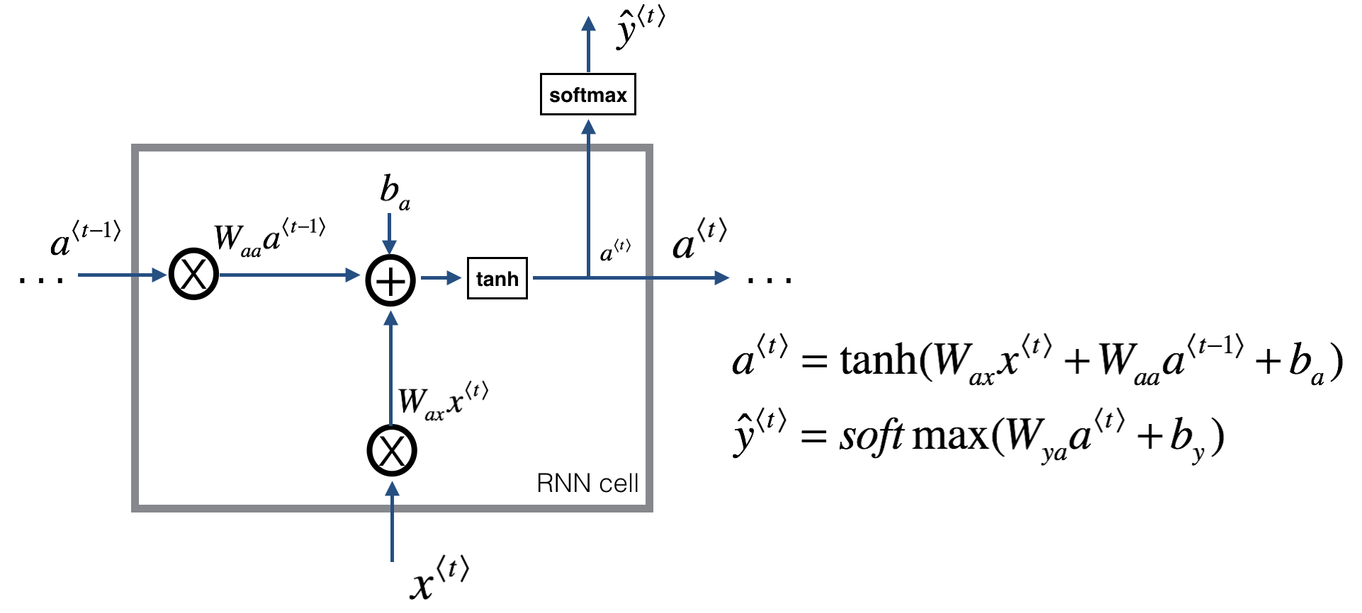
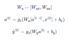
前向传播过程的公式如下：

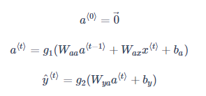
激活函数 g1通常选择 tanh，有时也用 ReLU；g2可选 sigmoid 或 softmax，取决于需要的输出类型。

为了进一步简化公式以方便运算，可以将 Waa、Wax水平并列为一个矩阵 Wa，同时 a⟨t−1⟩和 x⟨t⟩ 上下堆叠成一个矩阵。则有：(分块矩阵的写法，注意对应顺序。下图中 Wa 的写反了)

前向传播代码：

输入：xt 其中(n_x, m, T_x) n_x 为特征，m为样本数，T_x为时间步数

返回值：a_next, yt_pred, cache

中间值：因为反向传播需要，所以存储了 a_next, a_prev, xt, parameters

因为每个时间步共享参数，所以参数不变

# 单时间步
def rnn_cell_forward(xt, a_prev, parameters):
    """
    Implements a single forward step of the RNN-cell as described in Figure (2)

    Arguments:
    xt -- your input data at timestep "t", numpy array of shape (n_x, m).
    a_prev -- Hidden state at timestep "t-1", numpy array of shape (n_a, m)
    parameters -- python dictionary containing:
                        Wax -- Weight matrix multiplying the input, numpy array of shape (n_a, n_x)
                        Waa -- Weight matrix multiplying the hidden state, numpy array of shape (n_a, n_a)
                        Wya -- Weight matrix relating the hidden-state to the output, numpy array of shape (n_y, n_a)
                        ba --  Bias, numpy array of shape (n_a, 1)
                        by -- Bias relating the hidden-state to the output, numpy array of shape (n_y, 1)
    Returns:
    a_next -- next hidden state, of shape (n_a, m)
    yt_pred -- prediction at timestep "t", numpy array of shape (n_y, m)
    cache -- tuple of values needed for the backward pass, contains (a_next, a_prev, xt, parameters)
    """
    
    # Retrieve parameters from "parameters"
    Wax = parameters["Wax"]
    Waa = parameters["Waa"]
    Wya = parameters["Wya"]
    ba = parameters["ba"]
    by = parameters["by"]

    a_next = np.tanh(np.dot(Wax, xt) + np.dot(Waa, a_prev) + ba)
    # compute output of the current cell using the formula given above
    yt_pred = softmax(np.dot(Wya, a_next) + by) 
    
    # store values you need for backward propagation in cache
    cache = (a_next, a_prev, xt, parameters)
    
    return a_next, yt_pred, cache

# 多时间步
def rnn_forward(x, a0, parameters):
    """
    Implement the forward propagation of the recurrent neural network described in Figure (3).

    Arguments:
    x -- Input data for every time-step, of shape (n_x, m, T_x).
    a0 -- Initial hidden state, of shape (n_a, m)
    parameters -- python dictionary containing:
                        Waa -- Weight matrix multiplying the hidden state, numpy array of shape (n_a, n_a)
                        Wax -- Weight matrix multiplying the input, numpy array of shape (n_a, n_x)
                        Wya -- Weight matrix relating the hidden-state to the output, numpy array of shape (n_y, n_a)
                        ba --  Bias numpy array of shape (n_a, 1)
                        by -- Bias relating the hidden-state to the output, numpy array of shape (n_y, 1)

    Returns:
    a -- Hidden states for every time-step, numpy array of shape (n_a, m, T_x)
    y_pred -- Predictions for every time-step, numpy array of shape (n_y, m, T_x)
    caches -- tuple of values needed for the backward pass, contains (list of caches, x)
    """
    
    # Initialize "caches" which will contain the list of all caches
    caches = []
    
    # Retrieve dimensions from shapes of x and parameters["Wya"]
    n_x, m, T_x = x.shape
    n_y, n_a = parameters["Wya"].shape
    
    ### START CODE HERE ###
    
    # initialize "a" and "y" with zeros (≈2 lines)
    a = np.zeros((n_a, m, T_x))
    y_pred = np.zeros((n_y, m, T_x))
    
    # Initialize a_next (≈1 line)
    a_next = a0
    
    # loop over all time-steps
    for t in range(T_x):
        # Update next hidden state, compute the prediction, get the cache (≈1 line)
        a_next, yt_pred, cache = rnn_cell_forward(x[:,:,t], a_next, parameters)
        # Save the value of the new "next" hidden state in a (≈1 line)
        a[:,:,t] = a_next
        # Save the value of the prediction in y (≈1 line)
        y_pred[:,:,t] = yt_pred
        # Append "cache" to "caches" (≈1 line)
        caches.append(cache)
    
    # store values needed for backward propagation in cache
    caches = (caches, x)
    
    return a, y_pred, caches

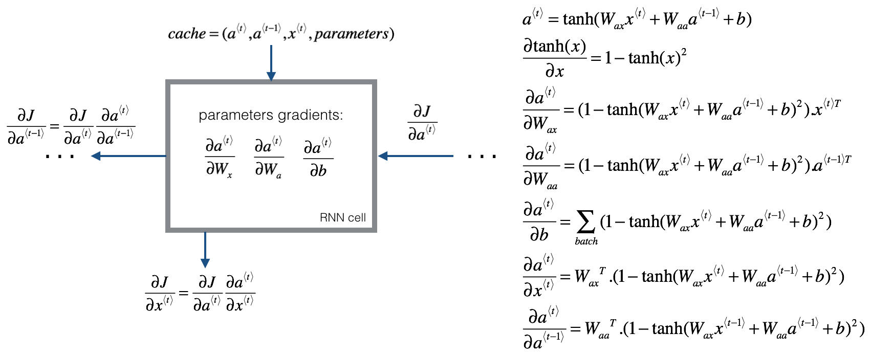
1.2 反向传播：

为了计算反向传播过程，需要先定义一个损失函数。单个位置上（或者说单个时间步上）某个单词的预测值的损失函数采用交叉熵损失函数，如下所示：

循环神经网络的反向传播被称为通过时间反向传播（Backpropagation through time），因为从右向左计算的过程就像是时间倒流。

更详细的计算公式如下：

1.3 梯度消失

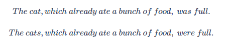
对于以上两个句子，后面的动词单复数形式由前面的名词的单复数形式决定。但是基本的 RNN 不擅长捕获这种长期依赖关系。究其原因，由于梯度消失，在反向传播时，很深的神经网络，从输出y^得到的梯度很难传播回去，很难影响靠前层的权重，后面层的输出误差很难影响到较靠前层的计算，网络很难调整靠前的计算。所以很难让它记住是单数还是复数。

在反向传播时，随着层数的增多，梯度不仅可能指数型下降，也有可能指数型上升，即梯度爆炸。不过梯度爆炸比较容易发现，因为参数会急剧膨胀到数值溢出（可能显示为 NaN）。这时可以采用梯度修剪（Gradient Clipping）来解决：观察梯度向量，如果它大于某个阈值，则缩放梯度向量以保证其不会太大。相比之下，梯度消失问题更难解决。GRU 和 LSTM 都可以作为缓解梯度消失问题的方案。

2 GRU

GRU（Gated Recurrent Units, 门控循环单元）改善了 RNN 的隐藏层，使其可以更好地捕捉深层连接，并改善了梯度消失问题。

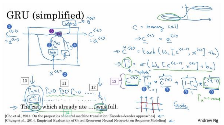
当我们从左到右读上面这个句子时，GRU 单元有一个新的变量称为 c，代表记忆细胞（Memory Cell），其作用是提供记忆的能力，记住例如前文主语是单数还是复数等信息。在时间 t，记忆细胞的值 c⟨t⟩等于输出的激活值 a⟨t⟩；c~⟨t⟩ 代表下一个 c 的候选值。Γu 代表更新门（Update Gate），用于决定什么时候更新记忆细胞的值。以上结构的具体公式为：

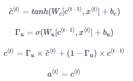
当使用 sigmoid 作为激活函数 σ 来得到 Γu时，Γu的值在 0 到 1 的范围内，且大多数时间非常接近于 0 或 1。当 Γu=1时，c⟨t⟩被更新为 c~⟨t⟩，否则保持为 c⟨t−1⟩。因为 Γu可以很接近 0，因此 c⟨t⟩几乎就等于 c⟨t−1⟩。在经过很长的序列后，c的值依然被维持，从而实现“记忆”的功能。

因为sigmoid的值很容易取到0，或者非常接近0，这时c(t)=c(t-1) ,有利于维持细胞的值。Γu很接近0，但不是0 ，就不会有梯度消失的问题了。有效缓解了梯度消失的问题。

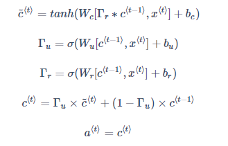
以上实际上是简化过的 GRU 单元，但是蕴涵了 GRU 最重要的思想。完整的 GRU 单元添加了一个新的相关门（Relevance Gate） Γr，表示 c~⟨t⟩和 c⟨t-1⟩的相关性。因此，表达式改为如下所示：

3 LSTM

LSTM（Long Short Term Memory，长短期记忆）网络比 GRU 更加灵活和强大，它额外引入了遗忘门（Forget Gate） ΓfΓf和输出门（Output Gate） ΓoΓo。其结构图和公式如下：